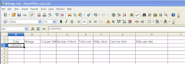
As promised the screen shot of the initial formatted spreadsheet, with the 12/03/10 example in the cell A3.
And Ooops a small error here, can you spot it?

For those of you who spotted it, you are observant, well done (the 'C' columm has not been widened sufficiently to see all the heading).
OK, now we will get into the remaining formatting. For this as there are a number of similar formatting items, we will go through it for the first instance and then you can finish the formatting in the remaining columns as per the table in the last blog item.
Right to set the 'B' column (mileage) to a number format with no decimal places, right click on the 'B' column header. Now left click on 'Format cells....'. From the 'Numbers' tab, left click on 'Number' under Category, then using the scroll bar (little blue up and down arrow heads) for the 'Decimal places' box (under the 'Options' section), set the value to '0'.
Note here you will also notice two tick boxes which when ticked (click in the box to make this happen), make either 'Negative numbers red' or 'Thousands separator' appear. You will also notice the 'Format code' area shows the invisible code which would be placed in the spreadsheet to make this happen.
A further point is the 'Leading zeros' option (setting this to '0' in the 'Leading zeros' box with the scroll bar would leave blank spaces in cells containing number formats - this is useful for those occasions where a cell contains a calculation, but no values to work with - we will see this later)
On to column 'C' and its setting for currency. This setting has an automatic two decimal place setting and the currency symbol of your choice (default is the country setting for your operating system - £ for UK, $ for US etc). So from the 'Format Cells' window (right click on column 'C' and select 'Format cells....'), left click on Currency and a number of options are automatically set for you (the negative numbers, thousands separator and their values). Left click on the 'OK' button.
The remaining columns are very similar in format, and with exception to column 'G', it will be a repetition of some the instructions above or in the last part of the previous blog. For the purposes of practice it will be left to you to set the formats for columns 'D', 'E', 'F' and 'H' (refer to the previous blog for the actual values and settings to make).
With column 'G' we have an additional formatting option, not seen in the others (setting the column and this includes the column heading 'Cost per mile' to a bold format). Once again, right click on column 'G', 'Format cells....'. Left click on the 'Font' tab, from here you can set the 'Font' style, its 'Typeface' and the 'Size'. Leave the 'Font' and 'Size' options as they are, but left click on the 'Bold' option under 'Typeface'. Left click on the 'Numbers' tab and set the values to 'number' and '2' decimal places.
To show what has been done put the following values into the cell shown (e.g. 4.83 [D3] means put 4.83 into cell D3)
26/07 [A3]
32098 [B3]
1.19 [C3]
29.7 [D3]
249 [F3]
We have missed out cells E3, G3 and H3 as these will be calculated (see below)
 |
| Mileage spreadsheet after formatting and adding dummy figures |
That's it for this time, see you next time
Prometheus1618
No comments:
Post a Comment