Impress - Open Office 3.30

Hi People

Last time we started work on the title slide for our slideshow.  So load it up (or create it as per the last post)

 It looks pretty basic at the moment so look at the picture below and we will work to producing this.

Firstly, choose another background, which is easily and quickly done, by looking to the right side column, under 'Tasks \ Master Pages'.  Look at the 'Available for Use' section (if you only see the grey bar with a '+' then left click on the '+' to expand the section - note the '+' turns to a '-').  Now click on the background you want to use.

Now lets add a picture, to do this, we will be using the 3 shape icon on the bottom toolbar (see picture below)

The bottom toolbar - below the main slide window

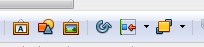
Here you can see the 3 shape icon (second from the left)

Click on the 3 shape icon and locate a suitable picture (perhaps one you have created or one from the internet - free of charge and royalties images only).  Select the image and then click the 'Open' button and wait a few seconds.  

The picture will arrive but not in the position you want to place it, see  the picture below

The picture was deliver in the centre of the slide, note the green  'handles' for re-sizing the picture

Place the mouse cursor in the picture and it will change to a cross with arrow tips.  Hold down the left mouse button and now you can move the picture to wherever you want to put it on the slide.  Use the green handles to resize the picture.  Play with this and get use to it as these handles appear on most containers to allow re-sizing.

Use the corner handles to reduce both height and width together, the mid line handles just re-size the sides, top or bottom (depending on which handle you use - use top for top etc). 

 To use the handles place the mouse cursor on the handle of choice (the cursor changes to a black outlined, white double headed arrow), and HOLD down the left mouse button, now move the mouse to resize the picture and let go of the button when you have got the width, height or width & height you want.

I have added a balloon callout to this slide

Ok from the picture above you can see I have added a balloon callout

 Callout from the bottom toolbar (4th icon in from the left)

Click on the black arrow tip to the right of the balloon (callout) icon and select (by left clicking on the shape you want).  The mouse cursor will now turn to a black cross when on the slide.  Position the cursor where you would like to put the callout  and HOLD down the left mouse button. Now move the mouse (while holding down the left mouse button) and the callout will form under the cursor as you move.  Note the callout has the green handles for resizing and a yellow handle which directs the length and direction of the callout source.

Click inside the callout and add the text you want to display.

Play with this and we will look at slide two and transitions next time

Thank You for stopping by Prometheus1618

Using Impress in OpenOffice - 3.30

Hi People,

Firstly, I want to apologise to those of you who were looking to create this slideshow some months ago.

Secondly, due to the time that has lapsed a newer version of OpenOffice and hence Impress (than the one I was originally using), is available.

My suggestion is that you, update your version of OpenOffice.org, so that we can all work through this together.

OK, there are some minor differences when you go through the sequence, of the several previous posts on the use of Impress.  The first major difference come with the button arrangement and what is shown on the menu.

The new Impress layout, with the original starter slide created.

So you can see that some button and options are not immediately available from the menu button directly.  For instance, we did have the ability to turn bullet points on/off via the default button bar.  This option is still available from the 'Format' menu, under 'Bullets and Numbering...' or you could create your own customised button bar with the buttons that you use most (we will look at this in a later post).

For now we will customise the toolbars by replacing the 'lines and filling' toolbar displayed (the one with the paint pot, pen nib, 0.00cm and the Black square in it), with the 'Text Formatting' toolbar.  This replacement tool bar has the Text justification, Font family, Font size, Bold, Underline, Italic and the Bullets buttons on it.
How to do this is:

• Click on 'Tools'
• Click on 'Customise' from the menu
• Click on the 'Toolbars' tab (at the top of the popup frame)
• Now, locate the 'Toolbar' box near the top (just under 'OpenOffice.org Impress Toolbars')
• Use the down arrow to the right of the box and the scroll bar, to select 'Text Formatting' toolbar.
• Click the 'OK' button and you will have the 'Text Formatting' buttons available on the toolbars.

Do not have too many toolbars available at any one time as these will crowd your monitor workspace.

Now if you have your 1st slide set up on the screen as above, perhaps we will 'tinker' with it. Firstly, let's have a much larger title 'Computer Parts' and let's centre it.   Centring the text can be achieved by setting the justification button to centre it looks like this

Before using the button, we first click once on the text in the box, this locates the editing cursor on the text, now highlight the text, by moving the mouse to the first letter of the title and holding the left mouse button down whilst moving the mouse over the entire text. Now where the toolbar shows the text size (see picture below) either type the size of the font (such as 36) or click the black down arrow to the right and select a size from the options.  In either case the highlighted text will change immediately in size.

Text Formatting toolbar showing Font, Font size (24 here), Bold , Italic,  Underline and  Shadow buttons

Now click the centre justification button as shown above.  This enlarged text is now centred.

Well that is it for now

Thank You for stopping by

Prometheus1618

We now have a FREE SPYWARE REPORT available, yours to keep and share if you wish. Fill in your details below and get yours now

eMail address:
First Name:

Using Impress - Part 3

Hi People

A Happy, Healthy, Wealthy and Abundant  New Year to you all.

OK now we were looking at a presentation using the Impress module of Open Office.

The slideshow we are creating is going to be about the parts of a computer.

Open your 'Slide test' presentation (if you haven't created it yet, have a look at the last couple of posts).

Firstly, if you want to change the background of your first page (and this can be achieved for all the pages if you want), select the 'Format' menu option, click on 'Page' and use the 'Background' tab.  I chose a blue background.

Now to title your slide,  double click on the 'My First Presentation' area.  Where you double clicked the cursor should be flashing and the 'My First Presentation' should be inside a box (if you have a box with 8 small boxes around the edge, you have single clicked by mistake).  Now you can delete, highlight and over type in the box.  So delete the contents and type in ' Computer Parts.

Similarly the 'Click to add an outline' box can be changed, so type 'A basic computer parts list'.  Now you may have a bullet list (a list with a large dot at the front).  To remove the bullet setup look to the icon bar and you should see an icon like the one below

The 'Bullet list' icon on the icon bar

If you click on it the bullets should disappear on the slide (make sure you are on the same line as the bullet you want to remove.  Question  How would you remove several bullets at once? Answer next time.

The 'justify' section of the icon bar. Note the 'left justify' icon is highlighted (in use). Use the 'centre justify' (the next icon right of the 'left justify'), by left clicking on it

You will also notice that the line is left justified, so again look to the icon bar and left click on the 'centre justify' icon.


Ok , now save your work an we will be looking at this further next time


Thank You for Stopping By


Prometheus1618



We now have a FREE SPYWARE REPORT available, yours to keep and share if you wish. Fill in your details below and get yours now

eMail address:
First Name:

Using Impess - Looking at the Options -1

Hi People

Last time we created our first slide (see last post if your unsure or haven't done this).  Also, there were a number of tabs in the main area to have a look at.  These add extra useful parts for the creator of the presentation.

The 'Normal' tab is where the slides are presented for creating and editing.
The 'Outline' tab shows the slides as thumbnails (tiny pictures) with the titles alongside
The 'Notes' tab displays any notes the presenter may which to add which are not seen on the slideshow/presentation
Predictably, the 'Handout' tab is for creating and editing a handout which can be generated to for presentation participants to take away as a hard copy.
Finally, the 'Slide Sorter', no prizes for guessing what this baby does (allows you to order  the slides to your preference of displaying them).  Now if you have checked these out while, going through the above list, you will notice the the 'Outline' tab does not have a right hand area sectioned off (Tasks area).

The remaining tabs do have the 'Tasks' area.  You have seen the 'Tasks' available from a 'Normal' perspective, so check out the remaining 'Tasks' on the 'Notes', 'Handout' and 'Slide Sorter' tabs.

What you will find is that they are all the same, allowing you to replicate your presentation effects over all (though how you could create transition effects on a handout is rather amusing).

That's it for this post

Thank You for stopping by

Prometheus1618

We now have a FREE SPYWARE REPORT available, yours to keep and share if you wish. Fill in your details below and get yours now

eMail address:
First Name:

Using Impress

Hi People

In the last post, we looked at the basics of starting an Impress presentation.  You may remember that, the Impress module of OpenOffice.org is the equivalent of Microsoft's PowerPoint.

In this post we will be creating a slideshow.  I am going to make this slideshow, purely for tutorial purposes.

The slideshow will be about computers and their parts and will be using pictures from various sources, just for illustration purposes.

The background is from an OpenOffice.org extension package called 'Modern-Templates.oxt' and is available here.

There are a few others contained in the extension for Impress.  To use it, just double left click the file and (assuming you have OpenOffice.org installed) it will install itself and show you a list of all the extensions you  have installed in OpenOffice.org.  To view the templates, you need to open Impress and look at the new templates individually.

OK open impress and go with the setttings as described in the last post.

The Presentation Screen with a single slide.  Note the Slide List on the left of the main work area and the Tasks area on
the right of the main work area

From the above picture of the presentation work area, you can see the menu and toolbars at the tops, the Slide list on the left, main work area,  and the Tasks area.  Below the Slides and Main area are the tool selection bar.

Note also the 5 tabs above the main area window (Normal, Outline, Notes, Handout and Slide Sorter)

Currently the Tasks area is showing the Layouts section.  Left click on the the other options

• Master Pages
• Table Design
• Custom Animation
• Slide Transition

The tool selection bar has a selection of options for creating your individual slides from scratch (or adding a little to existing slide layouts), for example various lines, shapes, connectors, symbols etc. and the ability to arrange them on the slide, by rotation, alignment etc.

Save your basic slideshow presentation as slidetest and we will continue in the next post

OK That's enough for now and we'll delve deeper next time

Thank You for stopping by

Prometheus1618

We now have a FREE SPYWARE REPORT available, yours to keep and share if you wish. Fill in your details below and get yours now

eMail address:
First Name:

Impress for the beginner

Hi People

Many will not know Impress (the presentation program within OpenOffice.org).  It is the equivalent of the Powerpoint presentation program within Microsoft Office.

Presentations can be made at all levels of social and business interaction, because laptop computers are now available to almost everyone.
Laptops are where most presentations are made from and so a party planner might put on a presentation, school children could watch a presentation (or even put one on), a returning holiday maker, may well put a presentation on for friends and family and of course a salesman may make a presentation to a prospect.

 These are some of the few possibilities, so getting to know what can be done with a presentation package can be very useful for many people.

Let's now take a look at Impress.  To open Impress for a new presentation, simply click on the OpenOffice.org icon and select the presentation icon or select Impress from the OpenOffice menu on All Programs.

In both cases a small wizard window opens and you can choose to use a blank or existing presentation or indeed use a template (leave the Preview box ticked). It is probably wise to use the wizard until you get to know your way around Impress.

Select the blank presentation then click the 'Next' button.

Now you may select the presentation background (it is very limited in the basic installation, but we will look at  getting new backgrounds  at a later time).  Select the Dark Blue with Orange.

Leave the 'Screen' box ticked as we are going to use a computer output presentation (The alternatives can be used for a printed output - Paper, an overhead projector - Overhead sheet or a slideshow projector - Slide).

Click 'Next' and now the options for the type of transition, its speed and a manual or automatic presentation are displayed.

Choose a transition type ( Effect ) and leave the Speed as medium and the Default radio button selected.

You can fill in the boxes on the next screen display if you wish, but they are not compulsory.

Now click the 'Create' button to begin creating your presentation proper.

That 's all until next time

Thank You for stopping by

Prometheus1618

We now have a FREE SPYWARE REPORT available, yours to keep and share if you wish. Fill in your details below and get yours now

eMail address:
First Name:

The Writer Experience

Hi People

At the end of the last post, I left you with an easy question.  The button you were looking for was the PDF button.

What are PDF well most people are aware that they are Portable Document Format files, but they are designed to be non-editable once published.  This means that you can provide them as 'fixed' documents. They are like a 'picture' of the text document.

OK, without a specific task in mind, let's see what we can do in Writer.

ITEM : How to create a header and footer in the document

With Writer open you will have your standard toolbars and menus.

Choose the 'Insert' menu item and the 'Header' item from the menu and from the submenu choose 'Default'

The top part of the page outline, splits into two.  The 'Header' portion and the, 'Body' portion.

This is like a page break, but it retains both sections on one page (and every page).

The footer can be created in a similar manner, using the  'Insert' , 'Footer' and 'Default'

The standard items you would find in a Header would be a logo, aside from things which may be put in alternatively in the Footer, such as the date, time, author initials, page count, total pages, addresses, email, telephone numbers, website addresses etc..  

Putting dates, times and  page count in the header or footer is done using the 'Field' menu item. Fields are found by using the 'Insert' , 'Field' and choosing the appropriate field to insert.

NOTE make sure you leave enough room ( vertically ) to get the recipient's address in, if creating  a header for a letter or letter template.

That's it for now

Thank You for stopping by

Prometheus1618














We now have a FREE SPYWARE REPORT available, yours to keep and share if you wish. Fill in your details below and get yours now

eMail address:
First Name:

Using Writer

Hi People

For the initial posts we have been looking at developing a couple of spreadsheets, so this time we are going to look at the Word compatible Writer module of OpenOffice.org.

It is a sophisticated document creating package, with the capability of saving the output to many types of format, notably :  .doc & .pdf


Most people will recognise both of these as being the formats used by Microsoft Word and Adobe Acrobat respectively.

So with out further explanation, let's dive in!

Open the Writer module, (either by opening the OpenOffice.org package and using the control panel, or by locating the Writer program in the programs list) and have a good look at the toolbars at the top.  Some of the buttons will be familiar (being the same or very similar to the ones in Word - excluding the new 'ribbon' arrangement in Office 2007 and 2010 - for Windows)

Writer's Toolbars

The lower of the two toolbars, has the standard options, such as

Font 

•  Size, 
• Style, 
• Bold, 
• Underline, 
• Colour 
• Type

Text

• Alignment (Left, Centred, Right and Justified)
• Indents, 
• Bullets,
• Highlighting

The remaining bar has a number of extra tools, most of which are found somewhere in Word, with one major exception.

I will leave you to figure out which tool button it is (clue - it is actually written on the button)

Thank You for your attention

Prometheus1618

We now have a FREE SPYWARE REPORT available, yours to keep and share if you wish. Fill in your details below and get yours now

eMail address:
First Name:

Personal Accounts - Conditional Formatting - Part 4

Hi People

The conditional formatting item is available on the 'Format' menu

The 'Conditional Formatting' option on the 'Format' menu

When you click on the 'Conditional Formatting' option, you will see the condition entry form

Several things to note here are

• the Condition 1 box is ticked, ready for the first entry
• there are 4 boxes of information required, to start with
• a maximum of 3 conditions are available

Click on the first box to change 'Cell value is' to 'formula is' 

When you change the 'Cell value is' to 'formula is', the middle box disappears, making way for a larger box into which you can type your calculation.  We are going to put the following calculation in

=OR(D7="d";D7="D")

The first calculation for the cell 

This will look familiar to you as it is one of the tests that make up the long calculation we studied several posts ago.  On clicking the 'New Style...' button you will find a window with 8 tabs.  Select the tab marked 'Background'

The 'Background' tab window

Select the red background for debits

Having selected the red background, by left clicking it, left click the 'OK' button and now left click in the 'Condition 2' box.  This will activate the second condition.

The two calculations for the conditional formatting styles (notice the third condition has not been activated)

Again change the 'Value is' to 'Formula is' and type in the formula

=OR(D7="c", D7="C")

Left click the 'New Style....' button and select a suitable green or blue color for the background of credits to the account.

Now left click the 'OK' button and let's test the results

From the picture below you can see what happens when you enter various credits and debits.

The final layout for the basic Home accounts program

Keep this spreadsheet handy as we will further develop it in a later post.

Next time we will look at the Writer program with Open Office.

Thank You for stopping by

Prometheus1618

We now have a FREE SPYWARE REPORT available, yours to keep and share if you wish. Fill in your details below and get yours now

eMail address:
First Name:

Personal Accounts - Conditional Formatting - part 3

Hi People

Let's have a look at the spreadsheet pictures and show you some of the things we have been discussing.

This picture shows the result of an unexpected value in D7.  See the WHAT! in F7

Notice here that the next entry still causes an error in the 'Balance' column - column F

When the errors are corrected, the system goes on working

In this picture a Credit or 'C' transaction is made, and the value of the balance goes up.  Whilst it has been tested the spreadsheet does need much more testing before being happy with the results being seen.

A large withdrawal here has caused the spreadsheet to use its internal conditional formatting.  The  -£17.17 in the 'Balance' column is in red numbers

The last picture above shows that some colour conditional formatting is used in the Currency format for numbers.  We can further enhance the conditional formatting if we wish.

We could highlight the transaction amounts if they are credits or debits for instance

Conditional Formatting is found under the 'Format' menu options, about half way down.

For what we are going to do is fairly involved, so the details we will leave until next time

Thank You for stopping by

Prometheus1618

We now have a FREE SPYWARE REPORT available, yours to keep and share if you wish. Fill in your details below and get yours now

eMail address:
First Name:

Personal Accounts - Conditional Formatting part 2

Hi People

The formula I left you with last time was quite large wasn't it.  Let's have another look at it.

=IF(E7="";"";IF(OR(D7="C";D7="c");E7+F6;IF(OR(D7="D";D7="d");F6-E7;"WHAT!")))

This formula has been entered as a replacement for the original formula in cell F7 (this is the 'Balance' column)

To break it down, I will highlight the parts as we go through them

First of all we check to see if cell E7 has anything at all in it (that is, it is not empty - note that a 'space' entry is not an empty cell), as is highlighted below.  Why do we check E7?  If E7 is empty then there is no transaction.

=IF(E7="";"";IF(OR(D7="C";D7="c");E7+F6;IF(OR(D7="D";D7="d");F6-E7;"WHAT!")))

Next we check if the cell E7 has an Upper Case 'C' or lower case 'c' in it. If it has then we add the content of E7 to the balance from F6.  Again this is highlighted below.  You will notice the use of the OR function which checks the entries inside the bracket for an entry which is true, if one or more are then the 'E7+F6' part is 'executed' (which means 'used' or 'run' or 'done').  If no entry is true then the next part of the calculation is done (which means 'used' or 'run' or 'executed')

=IF(E7="";"";IF(OR(D7="C";D7="c");E7+F6;IF(OR(D7="D";D7="d");F6-E7;"WHAT!")))

Now if the testing has got this far then a further check is made on the contents of cell D7 for an Upper Case 'D' or lower case 'd' (using the OR function again).   The highlighted section is the part to check out.
If a 'D' or 'd' is found then the contents of E7 are subtracted from F6.  Note that if the formula was E7-F6 we would get a very different - extremely different answer so make sure that you always check subtractions and divisions CAREFULLY or you could end up with some pretty weird results.  This was the second item you should have noticed from the end of the last post.

=IF(E7="";"";IF(OR(D7="C";D7="c");E7+F6;IF(OR(D7="D";D7="d");F6-E7;"WHAT!")))

Finally we have a SHOUT 'WHAT!' if the value is anything other than

• an empty cell
• a 'c' or 'C' entry
• a 'd' or 'D' entry

=IF(E7="";"";IF(OR(D7="C";D7="c");E7+F6;IF(OR(D7="D";D7="d");F6-E7;"WHAT!")))

If you see this check the column D entry and note also this will affect every entry in the F column after the error so it does continue to SHOUT at you.

That's all this time people

Next time we will look at a little inbuilt conditional formatting for colour etc..

Thank You

Prometheus1618

We now have a FREE SPYWARE REPORT available, yours to keep and share if you wish. Fill in your details below and get yours now

eMail address:
First Name:

Personal Accounts - Conditional Formatting

Hi People

In the last entry, we discussed the options for detecting debits and credits on our simple Personal Accounts spreadsheet.
And having decided on the extra column to make the user think about what is to be done, we require some alteration for the calculations in column F (after the insertion of the new column D), from F7 (not F6!) down.

Currently the calculation in F7 looks like this

=IF(E7="";"";E7+F6)

[ Note  how the values have been changed.
Before the insertion of the new D column the calculation looked like this
=IF(D7="","",D7+E6) ]

First of all we need to test the letter in column D for the letters C,c,D,d.  Any other entry should produce a bold error message.

You will notice that we check for capital C and normal c (Upper Case = Capital, Lower Case = normal) and also for Upper Case D and Lower Case d.  This is because we do not know if the user works with Upper Case or Lower Case letters, so we cover both possible entries.

The error message should be immediately obvious so I suggest a word all in Upper Case letters. I have chosen the word WHAT! to make it stand out.  We shall make it stand out even more later, with conditional formatting

OK take a look at the formula below.  Yes I think a number of you will experiencing a sharp intake of breath, but when broken down into its parts it is really quite simple.

=IF(E7="";"";IF(OR(D7="C";D7="c");E7+F6;IF(OR(D7="D";D7="d");F6-E7;"WHAT!")))

I am going to leave you with this formula to have a look at for next time and then we will break it down to show you what it means.  You will notice two things specifically (if your very sharp), one of which is not so obvious, but its effect would be alarming for the user.

Until next time, Thank You

Prometheus1618






We now have a FREE SPYWARE REPORT available, yours to keep and share if you wish. Fill in your details below and get yours now

eMail address:
First Name:

The Personal Accounts Spreadsheet continues

Hi People

Did anyone have a look at the possibilities for correcting the mistake over a debit being added to the balance, instead of taking it away from the balance.

Well there are a number of options here, two of which we will explore in more detail.

Firstly there is the use of minus values in the 'Amount' column, whenever a Debit is required (when money is taken away from the balance - this is known as a 'Debit'), the value must be put in with a minus sign to allow the calculation in the 'Balance' column to work correctly.

Using this method is going to require the user to make sure that the values are entered with the minus sign when required.  This will easily cause errors in entries as the minus sign will be forgotten, occasionally.

The second method will require the use of an additional column between the 'Type' and the 'Amount' columns.

This column will be used to put the letter 'D' or 'C' into the appropriate row.  The letter entered will be tested, and one of three outcomes will  result in either the Balance being credited (added to), debited (reduced) or NO Change (if any other letter or character other than 'C' or 'D' is placed in the cell).

This is the method we will adopt as it will provide some 'error checking' as well as a thought provoking entry in the new 'D' column

We will make this more obvious by using 'conditional formatting' to colour the amount depending on a '(D)ebit, (C)redit or error input (any other letter, number or character - apart from no value - that is no entry)

Are we ready to do this?

Place the mouse pointer over the boundary line between the C and D columns ( that is at the top of the columns), this will create a double headed arrow if you have in the right place.  Now RIGHT click and select 'Insert columns' and a new empty 'D' column.

All the calculations have been automatically changed to make sure they work as they did before the column was inserted.

We will change the calculation in the Balance column to create the right result for debit and credit transactions and this will be looked at next time


Thank You

Prometheus1618



We now have a FREE SPYWARE REPORT available, yours to keep and share if you wish. Fill in your details below and get yours now

eMail address:
First Name:

Personal Accounts - Layout 2

Hi People

Been a while, but let's get down to it, you will remember that I left you with the task of playing with the formatting for the Title.  The merged block of cells at the top of the spreadsheet.

Following on from the basic formatting, let's sort out the formulae (plural of formula i.e. calculation).

Initially we want a balance to start the proceedings. So we will put the initial value of 0 in G5 (or you can put your own value in here). And  dont forget to format the cell as currency.

The Spreadsheet so far showing the starting balance of £0.00 (after formatting the cell for currency)

Now the cell E6, will contain a formula which will be unique to that cell, as it will be referring to the G5 cell, where as the remaining column calculations will be based on the cell above (e.g. the calculation in E7 will refer to E6 as the balance).

OK the calculation for cell G5 is:

=if(D6="";"";D6+G5)

The cell below will contain the formula

=if(D7="";"";D7+D6)
See below

This is the spreadsheet with the formulae entered (which would be blank without any values entered)

Looking at the picture above I have put 2 entries into the spreadsheet, showing  the calculated values, which as you can see, incorrectly calculates the cash debit on row 7. 

 The value is added to the balance from D6 instead of reducing the balance.  

Clearly we need to do something about this.  

Think about it and we will deal with this issue next time

That's all for now

Thank You

Prometheus1618

We now have a FREE SPYWARE REPORT available, yours to keep and share if you wish. Fill in your details below and get yours now

eMail address:
First Name:

Personal Accounts - Layout 1

Hi People

Let's do more with the Personal Accounts spreadsheet we started last time.

First though, you may have noticed that when you start a new spreadsheet, the program always starts with 3 sheets.  This is a situation which requires a new spreadsheet to correct but we will deal with that another time.

The extra sheets can be removed in the current spreadsheet by RIGHT clicking on the tab you which to remove (the tabs are at the bottom left hand side of the spreadsheet)

A Tab at the bottom of the spreadsheet, normally there are three

Select 'Delete sheet...' from the menu and 'yes' when prompted.

Sheet gone and job done.

Also you can 'Rename' the sheet from the same menu (as I have done in the above picture).

Continuing with your spreadsheet, currently it has a very basic layout, so let's change the appearance a bit.

Highlight row 5 (left click on the 5 on the left side of the spreadsheet) and click the centre alignment button on the Formatting Tool Bar (This is the bar with the 'Default' , 'Arial' font and '10' font size boxes at the left of the  toolbar - see below)

The left hand part of the 'Formatting' Toolbar, showing the 'Default'  format setting, the 'Arial' font setting and the '10' font size'

The 'Centre text horizontally' button

Now your headings are all centred.

To make a bit more of the top of the spreadsheet, how about a nice big heading in a merged block of cells.  To merge the cells, highlight the block from B2 to F3 ( that is two rows and four colums), now press the 'Merge Cells' button

The 'Merge Cells' button

The range will now be a merged block.  Click inside the merged block and set the font size (see the picture above) to 18.  Now create you own heading or you can stick with 'My Accounts' as I have done. 

You can also set the title as centred. and let's add a bit of colour, by right clicking in the merged block of cells and selecting 'Format Cells....' from the list.  

The 'Background' tab is the one you want and select a colour of your choice. 

Also play around with perhaps making the headings bold and adding a coloured background.

Have a go and we will have a look at it next time.

Well that's it for now.

Thank You for your attention

Regards

Prometheus1618

We now have a FREE SPYWARE REPORT available, yours to keep and share if you wish. Fill in your details below and get yours now

eMail address:
First Name:

Personal Accounts Spreadsheet

Hi People

Following on from the basic Mileage spreadsheet, and with no suggestions as yet as to what you would like to see as a spreadsheet project, I felt a Personal Accounts spreadsheet, might be of use.

I would however, ask you to look over ALL the first tutorial as I will be making some assumptions on what you know, based on information from the earlier tutorial.  So please review the last tutorial fully, before getting into this one.

OK that being said (also I would like to add, that I cannot ANY responsibility for your use, misuse or abuse of this information or any errors which may creep in), let's get going.

Open OpenOffice Calc and  setup the following  in row 5 (these are the headings)

Date (B5) means put the title 'Date' in cell B5

So

Date (B5), Transaction (C5), Type (D5), Amount (E5), Balance(F5)

These will do for now we may add more columns later.

If you remember how to set Formats for the individual columns (check back to the last tutorial for more information), set the column B as a Date format, set columns E and F as currency

For now that's it

See you next time
Prometheus1618



We now have a FREE SPYWARE REPORT available, yours to keep and share if you wish. Fill in your details below and get yours now

eMail address:
First Name:

Tidying up the Spreadsheet - part 2

Hi People

Last time we created a 'nested' IF formula for the cell range G4 to G20.  It solved the issue with the '#VALUE!' display if there was no value in the E4, E5 .... or if F4, F5 .... contained a "value too small" result.

Following this I requested that you have a go for yourself at creating a similar formula for the H4-H20.
Did anyone do it?

OK, Good on you if you had a go and it didn't quite work.
Keep it up and you will get there.

Brilliant, if you did and it worked, you're getting the hang of this whole spreadsheet thing.

ALWAYS test your spreadsheet for common errors at least, but if you can test it for all sorts of errors you can come up with.  This will make it more robust to the user.

The formula, I came up with for cell H5, was
=IF(D5="";"";IF(F5="value too small";"";F5/D5))
 
[ See how similar it is to the one in G5
=IF(E5="";"";IF(F5="value too small";"";E5/F5)) ]

We are checking, first of all, that there is no value in D5, if there is no value then we display no value (nothing represented by "").

 If there is a value in D5, then we check the F5 cell for "value too small", if there is a "value too small" result then nothing is displayed, if the F5 cell contains an acceptable value, then H5 will contain the result of F5/D5.

You will also notice in this formula that both the cells used in the final calculation are tested for values.

Covering your 'exceptions' like this are normal, when creating a spreadsheet, as they frequently pop up, due to the user mis-typing or not understanding what value types (or ranges - we will look at these sometime too) are supposed to be in the cells to get the calculation to work.

Now clearly you cannot cover all possible errors, but the main ones should be covered either by providing error messages (such as the "value too small" message), or a no entry, where excessive error messages may appear.  

Note that too many error messages may well hide the original error, from untrained eyes.

We will look at further error handling in future, but for now that is it for this post

Thank You for your company, and see you next time

Prometheus1618




We now have a FREE SPYWARE REPORT available, yours to keep and share if you wish. Fill in your details below and get yours now

eMail address:
First Name:

Tidying up the Spreadsheet

Hi People

In the last post we were testing the spreadsheet, when a couple of incorrect inputs threw up a " #VALUE! " error in the G5 and H5 cells.

How can we get around this?

Well one solution would be to test one of the cells which throw up the error, or you could test to see if the result of a calculation produces an exception error.

This is the approach we will adopt here, as then we cover the possibility of E4 containing nothing and F4 having a value too small ( this means a negative value being produced in F4).

So take a look at the formula below

=IF(E4="";"";IF(F4="value too small";"";E4/F4))


There are two conditional IF statements, one of which is only checked if the first IF statement is FALSE.

Remember that the basic format for an IF conditional formula is

=IF(Test;True Result;False Result)

So to explain this, the above says IF the Test is True then use the True Result, but IF the Test is False then use the False Result.

OK enough of the revision.

  Our new formula (which is put into cell G4) says:
IF the value in E4 equals Nothing ( "" ) then the True result equals Nothing ( "" ), but IF there is a value in E4 then process the second IF fornula.

Which reads as

IF the value in F4 equals "value too small" (the value has to equal the quote exactly, but as we put the value as a result to an earlier calculation, this is going to be a known result) then the True result equals Nothing ( "" ) but IF there is a value in F4 then put the True result ( in this case the  result of a calculation F4 / F4 ) into the cell.

If you put this formula into G4 and use the 'black box' method to copy the the formula, this will deal with the possible " #VALUE! " display in the G column, but can you use the above information to create a formula for the H column?


We will go through this next time


Also if there are any suggestions for another spreadsheet you would like to see developed, please leave a comment and we will go through the most popular request.


Thank You for your attention


Prometheus1618





We now have a FREE SPYWARE REPORT available, yours to keep and share if you wish. Fill in your details below and get yours now

eMail address:
First Name: