Winding up the Mileage spreadsheet part 2

Hi People


From the last post, we  were looking at the formula  below (if you cannot remember have a look at the previous blogs).  The formula was created in cell F4 (in the explanation below it is called the 'target cell').


=IF(B4<>"";IF(B4>B3;B4-B3;"value too 


small");"")


The formula below highlights the TEST1, TRUE1, FALSE1 parts of the formula by underlining the parts 


Test1


=IF(B4<>"";IF(B4>B3;B4-B3;"value too 


small");"")   




True1


=IF(B4<>"";IF(B4>B3;B4-B3;"value too 


small");"")




False1


=IF(B4<>"";IF(B4>B3;B4-B3;"value too 


small");"")  


Ok so verbally what this formula says:
TEST (underlined Test1 section)
IF the contents of cell B4 is NOT EQUAL ( '<>' is a NOT EQUAL sign) to NOTHING (remember  that two quote marks - without a space between - is NOTHING)


IF the above condition is TRUE (True1 underlined section) then calculate the second IF test (we will go througn this below)


IF the above condition is FALSE (False1 underlined section) then the contents of B4 are set at "" (nothing).


Now onto the second IF Test in the formula (remember for the second test to be calculated, the first test must be True).


Test2


=IF(B4<>"";"";IF(B4>B3;B4-B3;"value 


too small");"")




True2


=IF(B4<>"";IF(B4>B3;B4-B3;"value too 


small");"")




False2


=IF(B4<>"";IF(B4>B3;B4-B3;"value too 


small");"")


The underlined section  (Test2) above states that if the contents of cell B4 is GREATER THAN the contents of B3


If the Test2 is True then True2 will be adopted and the cell contents will contain the value left after taking the contents of B3 away from the contents of B4  (e.g.  IF B4 contains 38800 and B3 contains 38400 then the target cell - the cell which contains this formula - will end up with 38800-38400 = 400 as its contents.


If the Test2 is False then False2 will be displayed.  The cell will contain the words 'value too small' as a warning that the value in B4 is lower than that in B3.  Note here that words are enclosed in quotation marks "value too small" in the formula.


We will play with the spreadsheet in the next session.


Until then


Thank You for your attention


Prometheus1618


We now have a FREE SPYWARE REPORT available, yours to keep and share if you wish. Fill in your details below and get yours now

eMail address:
First Name:

Winding up the Mileage spreadsheet part 1

Hi People

Your  spreadsheet is now taking shape, enter the two remaining formulae as shown below, to make sure that when you copy the formulae (by the way formula is singular i.e  1 formula  2 or more are formulae) down the appropriate column (from row 3 to row 20).

For column G  we put

=if(E3="";"";E3/F3)
And using the little black box method to copy the formula to cell G3 to G20

For column H we put

=if(D3="","",F3/D3)
Again copy the formula to cells H3 to H20

There is one thing which we can do, to make things a little easier for you.  When you put in your mileage, from the start mileage you need to find out what the second mileage is and then subtract the start mileage from the second mileage.

This might be easier to explain with an example.

You decide to find out how many miles you do between filling up at the fuel station.

What you need is a full tank to start and the start mileage.  Now you cannot work out anything until you fill up with fuel again and get second mileage.  Once you have both, you can find out how many miles you have travelled and how many litres of fuel you have used.

So having put the start mileage into the spreadsheet, you cannot work out anything until the next fuel fill up and  mileage reading.  Therefore only cells A3 and B3 can have a value when you start using this spreadsheet.

On the next fill up you have your second mileage which can be used (by the spreadsheet) to calculate (yes I said calculate) the miles done.

To do this put in cell F4

=IF(B4<>"";IF(B4>B3;B4-B3;"value too small");"")

See if you can work out what is going on here (hints:  The '<>' is a 'not equal' sign , the '>' is a 'greater than' and look for 2 conditional if calculations one inside the other)
We will go through it together next time.

Until next time Thank You


Prometheus1618





We now have a FREE SPYWARE REPORT available, yours to keep and share if you wish. Fill in your details below and get yours now

eMail address:
First Name:

Formula explanation

Hi People

The last post was a little lengthy and a number of new concepts (for a total beginner)

The formula which we left off at was the one below

= if (d3="";"";c3*d3)     remember that c3 is the same as C3 etc

OK, now remember that ALL calculations start with an '=' sign, so that part is standard with any calculation.

The ' if ' part is the most common way of setting a conditional calculation. The format is

=if (something is true; do this ; if false do this)
There are 3 parts to this calculation

1. The test - in our equation we are testing if there is anything in cell d3
2. True option - if the content of d3="" then display "" (the double quote marks with nothing - not even a space - are the same as saying nothing) so the test is saying if d3="" (nothing) then put "" (nothiing) in this cell.
3. The false option - if the content of d3=3 (clearly there is something there now) then multiply the contents of c3 by the contents of d3 and put the result in this cell.

Can you figure out what to do for the other two  calculated columns (only g3 to g20 and h3 to h20 need to be used for the moment).

That is all this time people

Thank You

Prometheus1618

We now have a FREE SPYWARE REPORT available, yours to keep and share if you wish. Fill in your details below and get yours now

eMail address:
First Name:

Formatting - 3 and Formulae

Hi People

We are nearly at the end of our formatting on the spread sheet, all that we want to do now is make the column headings all bold.  To do this left click on the number 2 (indicating the second row) on the left hand side of the spreadsheet, highlighting the whole row.  Now simply look to the formatting toolbar for the B button (See Below) and left click on it, the effect is to make all in the row BOLD.

The 'B'old button

Formulae


Now to the more interesting side of the spreadsheet creation, the formulae.


Let's get into the first.one


Left click in the E3 cell, now type in exactly as shown below and we will go through it after.


=C3*D3

Here you can see the calculation being entered - at this point the 'Enter' key has not been pressed

Now for the explanation, all formulae start with an '=' sign, this lets the Calc know that what follows is a calculation.  These can be simply calculations, such as the one we have just typed in, or a conditional one (one of several outcomes), or very complex multiple formulae.

OK so back to the formula (calculation), the C3, and D3 labels are clearly referring to the cells C3 and D3.
It may be no shock to any of you at the '*'  (to get this character hold down the 'Shift' key -sometimes just an up arrow - and press the '8' key on the top row of the keyboard) is a multiply symbol.  So this formula just multiplies the C3 content by the content of D3 and puts the result in E3.

An example would be C3 contains £1.10 and D3 contains 30.0

The result is      £33.00

Now to G3
=E3/F3

I am sure you can work out what is going on here.  The differences from E3 are that this one uses the result of another calculation (E3) and the use of the '/' for division (E3 used the '*' multiply sign)


An example would E3 contains £33.00 and F3 contains 100


The result is    £0.33


Finally H3 is

=G3/D3

No explanation needed here as it is very similar to G3

The remaining formulae have been added here - note that the cell g3 contains a bold result, this is because we set all of column G to be bold in our formatting session.

So that is the basic formulae created, but how to create the same formulae down the sheet, with the right cells being used.  Spreadsheets, are designed to calculate and multiple similar calculations are a feature of most spreadsheets.  They have an easy method of replicating cell formulae.

To replicate the formula in E3 down the E column to E20, simply left click on the E3 cell and you will notice that the cell border becomes black and a small black square on the bottom right corner appears (see below). Left click and hold the left mouse button down on this little black square.  Now drag the square down the E column to cell E20.  Now you can let go of the button.  The E column from E4 to E20 now has £0.00 in the cells.

The mouse pointer, pointing at the 'black box/ for copying formulae down the column (or across the row)

Copying the initial '=C3*D3' formula to give a column of £0.00

This looks untidy, and the astute amongst you may remember that the formatting of numbers allowed you to turn off the leading zero, but unfortunately this does not work leaving £.00 in the cells instead. 

 There is a slightly more complex formula we can use instead of just


=C3*D3

The upgraded formula is a conditional formula as shown below

=if( D3=""; "";C3*D3)

Put this in the E3 cell, to do this you will need to remove the existing formula, so left click in E3 then press the delete key on your keyboard.  A 'Delete Contents' window opens and for now just hit the 'OK' button.

What pressing the 'Delete' key does in Calc

Now type the  formula below into the E3 cell exactly as you see it 

=if( D3=""; "";C3*D3)                                                   

Note that the separators are ' ; '  and not ' , ' or ' : '    (Excel uses the ' , ' )

Putting in the conditional formula

 Once that is complete, use the black square on the bottom right hand corner of the E3 cell to copy the formula to all cells down to E20.  The cells will now show nothing until the appropriate D cell has a value.

After the conditional formula has be added to cells E3 to E20 - Note the little black box

Have a think on this and next time we will go through the reasoning for this and how it works.

Thank You

Prometheus1618



We now have a FREE SPYWARE REPORT available, yours to keep and share if you wish. Fill in your details below and get yours now

eMail address:
First Name:

Your First Open Office Spreadsheet - Part 3 - Formatting 2

Hi People,
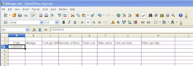
     As promised the screen shot of the initial formatted spreadsheet, with the 12/03/10 example in the cell A3.
And Ooops a small error here, can you spot it?

For those of you who spotted it, you are observant, well done (the 'C' columm has not been widened sufficiently to see all the heading).  

OK, now we will get into the remaining formatting.  For this as there are a number of similar formatting items, we will go through it for the first instance and then you can finish the formatting in the remaining columns as per the table in the last blog item.

Right to set the 'B' column (mileage) to a number format with no decimal places, right click on the 'B' column header.  Now left click on 'Format cells....'.  From the 'Numbers' tab, left click on 'Number' under Category, then using the scroll bar (little blue up and down arrow heads) for the 'Decimal places' box (under the 'Options' section), set the value to '0'.  

Note here you will also notice two tick boxes which when ticked (click in the box to make this happen), make either 'Negative numbers red' or 'Thousands separator' appear.  You will also notice the 'Format code' area shows the invisible code which would be placed in the spreadsheet to make this happen. 

A further point is the 'Leading zeros' option (setting this to '0' in the 'Leading zeros' box with the scroll bar would leave blank spaces in cells containing number formats - this is useful for those occasions where a cell contains a calculation, but no values to work with - we will see this later)

On to column 'C' and its setting for currency.  This setting has an automatic two decimal place setting and the currency symbol of your choice (default is the country setting for your operating system - £ for UK, $ for US etc).  So from the 'Format Cells' window (right click on column 'C' and select 'Format cells....'), left click on Currency and a number of options are automatically set for you (the negative numbers, thousands separator and their values).  Left click on the 'OK' button.

The remaining columns are very similar in format, and with exception to column 'G', it will be a repetition of some the instructions above or in the last part of the previous blog.  For the purposes of practice it will be left to you to set the formats for columns 'D', 'E', 'F' and 'H' (refer to the previous blog for the actual values and settings to make).

With column 'G' we have an additional formatting option, not seen in the others (setting the column and this includes the column heading 'Cost per mile' to a bold format).  Once again, right click on column 'G', 'Format cells....'.  Left click on the 'Font' tab, from here you can set the 'Font' style, its 'Typeface' and the 'Size'.  Leave the 'Font' and 'Size' options as they are, but left click on the 'Bold' option under 'Typeface'.  Left click on the 'Numbers' tab and set the values to 'number' and '2' decimal places.

To show what has been done put the following values into the cell shown  (e.g.  4.83 [D3]  means put 4.83 into cell D3)

26/07 [A3]

32098 [B3]

1.19 [C3]

29.7 [D3]

249 [F3]

We have missed out cells E3, G3 and H3 as these will be calculated (see below)

Mileage spreadsheet after formatting and adding dummy figures

That's it for this time, see you next time

Prometheus1618

We now have a FREE SPYWARE REPORT available, yours to keep and share if you wish. Fill in your details below and get yours now

eMail address:
First Name:

Your First Open Office Spreadsheet - Part 2 - Formatting -1

Hi People

To continue with our 'Car Mileage' project in Calc (part of the free OpenOffice.org suite), let's now turn our attention to some basic formatting of the spreadsheet. Formatting is the changing of the appearance or reaction of the columns, rows or cells affected by the formatting.

Column Formatting

Firstly, for the widening of the columns. To do this simple move your mouse pointer to the join, between the column headers, on the right hand side of the columm header, you want to widen. The pointer will turn to a double headed black arrow (the points are at either end of the horizontal bar). 

 Now press and hold down the left mouse button (whilst the pointer is still the double headed black arrow) and move the mouse to the right on the right hand side of the column header. This will widen the column (moving the mouse pointer to the left narrows the column). 

You will have noticed the tool tip pop up indicating the width of the column (this changes as you widen or shorten the column width).

Here is a short cut to setting the column to the maximum width to show the longest entry in the column. Again move the mouse pointer to the right hand side of the column you want to set (double black arrow). Now quickly double click and the header will respond to widen or shorten the width of the column to display the longest entry in that column.

Another shortcut to adjust the width of a number of columns together (and have the same width).

Choose your start column header and hold down the left mouse button, now move the mouse pointer over the column headers until you have reached the last one in the group you want to adjust.

From here it is a simple 'double black arrow' routine (as described above) and the columns respond accordingly once the mouse button has been released.

Just to recap to highlight a column, simply left click on its column header (the one with the letter in it), the column and its header now turn blue indicating that it highlighted. For a range of columns, hold down the left mouse button while the mouse pointer is on the first column header in the range and move the mouse pointer to the last column header, you will now have a sequence of blue highlighted columns.

 Try the double click column adjustment to a range of highlighted columns, magic, they all respond to the maximum length entry.

Now rows are somewhat similar to columns (except they are across the spreadsheet instead of down ), so you can now use the above to do a little experimenting with the rows. Make sure you have the original spreadsheet saved, then play with the rows and columns. Do not save it if you are playing unless you use the 'save as' option from the File menu and CHANGE the filename – just add play to the name and save.

Further formatting can be applied to complete columns.

We are going to format the following columns to the settings that follow the column letters:

Column   Settings
A            Date, centred across the cell
B            Number (no decimal places)
C            Currency (this is number and two decimal places + a currency symbol)
D            Number (with one decimal place)
E            Currency
F            Number (no decimal places)
G           Currency, in bold font
H           Number (with 2 decimal places)

So, to get the column A to show dates in date format, left click the column header, to highlight it.

Now without moving the mouse pointer, right click and select 'Format Cells …' , then select the 'Numbers' tab by left clicking on the tab name.

There are a number of selections and entry points here. Under the 'Category' heading, follow the list down to 'Date' and left click on it. Now on the 'Format' heading left click on the most appealing data format for you (though we suggest the dd/mm/yy - shown as 31/12/99 - format for now).

The box to the left bottom, shows a sample of the format chosen, so try several and watch it change, then return to the dd/mm/yy format by left clicking it.

Please left click on the 'Alignment' tab, to shown the column alignment settings. Under 'Horizontal' area within the 'Text alignment' section, left click on the blue'V' at the left hand end of the box which probably shows 'Default'. From the drop down list, left click on 'Centre'.

Left click the 'OK' button, this will return you to the spreadsheet, with the A2 cell text centres and no other shown differences, but try this left click in cell A3, type in exactly 12/03 and press enter, whatever date format you chose will show up. If it was the 'dd/mm/yy' format, then the /10 will be added to the end, also the date will be centred in the cell.

We will continue this formatting in the next item - with a picture of how it should look at this point.

Until then people, any questions, queries or comments, please leave them in the comments section below

Prometheus1618

We now have a FREE SPYWARE REPORT available, yours to keep and share if you wish. Fill in your details below and get yours now

eMail address:
First Name:

Your First Open Office Spreadsheet - Part 1

Hi People

Now you have got your OpenOffice.org program up and running (You haven't, see last post on this blog), we can get our first file created. A spreadsheet is what I have chosen to start.

Sometime soon, we will be adding video clips to give a little more information , but for now its just the text and snapshots.

Open your OpenOffice program. Select 'Spreadsheet' (Very similar to Excel in look isn't it?).
The spread sheet will be centred around getting you Mileage calculated and costed for you, so we will call it "Car Mileage" OK.

Firstly nearly the whole screen is covered in little blocks, these are called cells. Cells are the basic blocks (no pun intended) of the spreadsheet. A spreadsheet contains a number of these cells. Each cell is called by its Column Letter and Row Number. So if you wanted to put the word 'Miles' into D5. First find the column headed with D and follow it down until you come to row 5. Left click in this cell. This would place the cursor in that cell. Now you can type Miles into that cell.

Headings for Columns:

We will need the following headings (initially)
Date [A2]
Mileage [B2]
Cost per litre [C2]
Number of litres [D2]
Total Cost [E2]
Miles [F2]
Cost per mile [G2]
miles per litre [H2]
litres per 100km [I2]



If you put these headings in the cells in the [ ], so that for example Miles will go into cell [F2].  You may need to widen some columns (we will do that next time if you cannot figure out how to do it).

Now we need to save the the spreadsheet, left click on File (top left of screen ) and find and left click on Save in the the menu list.  The 'Filename' box should have 'Untitled 1' highlighted in blue, just type Mileage (you don't have to clear the box first).  Under the 'Filenname' box, you will see a box with 'Save as type' to the left of it and 'ODF Spreadsheet  (.ods)' in the box.  Left click on the blue 'V' to the right of the box and select 'Microsoft Excel 97/2000/XP (.xls)'.  Now left click on the 'Save' button. Job done - you will find the spreadsheet in your 'My documents' folder.
That will be all for this time, people, but I will leave you to think on what columns we are going to put our dates, and figures into and what columns are going to be worked out by the spreadsheet.

See you next time
Prometheus1618


We now have a FREE SPYWARE REPORT available, yours to keep and share if you wish. Fill in your details below and get yours now

eMail address:
First Name: